Intro

There is a lot of publicly available gene expression data out there. Despite the data being ubiquitous and free, these millions of samples are infrequently used. Instead, a typical study design looks something like

1. Collect samples for a condition of interest
2. Sequence gene expression for the samples
3. Find which genes are differentially expressed in the cases vs the controls
4. Run some other experiments and publish a paper
5. Toss the gene expression data into the pile labeled “SRA” and move on

That’s not to imply that this is a flawed study design. It does exactly what it’s intended to — it tells you which genes are up/downregulated in the samples. But wouldn’t it be nice to put that into biological context?

Enter PLIER. PLIER keeps the nice aspects of PCA while taking steps to avoid the “all your PCs are different flavors of batch effects” result that can happen when using PCA on expression data. This article describes what PLIER is, how PLIER works, and some applications described in the MultiPLIER paper.

PLIER

The idea behind PLIER is to “infer a biologically grounded data generating model that provides estimates of underlying biological processes, including explicitly identified pathway-level and cell-type proportion effects” using matrix decomposition. If that description made sense to you, you can probably skip to the methods section. If you’re like me, and there are several things in that sentence that didn’t quite parse, read on.

In non-technical terms, PLIER finds a small number of explanations (called latent variables) for a large number of changes in gene expression. In doing so, it makes three main assumptions:

1. There are, in fact, a small number of factors that explain changes in gene expression (a.k.a. the manifold hypothesis)
2. Good explanations are likely to be related to known biological pathways and genesets
3. The relationships between the explanations and the gene expression are linear

The Manifold Hypothesis

The manifold hypothesis is the assumption that a high-dimensional space can be modeled by a low-dimensional one. Since the term “dimensionality” will come up frequently, it’s worth being more explicit about what it means. In this usage, “dimension” refers to how many numbers it takes to describe a data point.

Gene expression is described as high-dimensional because a single sample has tens of thousands of genes. Is it really necessary to know the expression of every gene, though? Probably not. If you were working with bacteria, you could have a latent variable called “lac repressor level” that would describe how much expression you’d expect from multiple lac genes.

Pathways

While it can be helpful to describe gene expression in a small number of variables, which variables you use is critical. If you have four samples, you could memorize the expression and describe it with one variable (‘which sample is the gene expression from’). Similarly, technical artifacts like batch effects make good predictors of gene expression that are useless outside the original dataset.

We want a model of gene expression that describes future data, so spurious predictors won’t do. The novel contribution of PLIER is to steer the model away from spurious predictors by grounding the model with prior biological knowledge. In the next section, I’ll go into more detail to explain how they accomplish that.

Linear Relationships

The assumption that relationships are linear is both probably untrue and probably useful. Gene expression regulation isn’t really a linear process, i.e. 2 more molecules of inhibitor != 2 fewer rounds of transcription. That being said, because there are so many genes that need to be described, using a more complicated model may not be helpful¹.

How does PLIER work?

There are a lot of details and a lot of math that go into making PLIER work. The summary is that PLIER creates a model that transforms gene expression data into latent variable measurements by:

1. Maximimizing how well the latent variables can recreate the original data, while
2. Encouraging the latent variables to look like genesets,
3. Encouraging the weight of each latent variable to be small, and
4. Encouraging each latent variable to correspond to one or few genesets.

If that makes intuitive sense, feel free to move on to the applications section. Otherwise, here is a more in-depth description.

How does PLIER really work

PLIER uses matrix factorization, so understanding PCA/matrix factorization more generally will help understand this section. I explain the process in terms of finding explanations for data, but other interpretations like rotating the data or minimizing variance may make more sense to you.

The best starting place for understanding PLIER itself is probably the figure below.

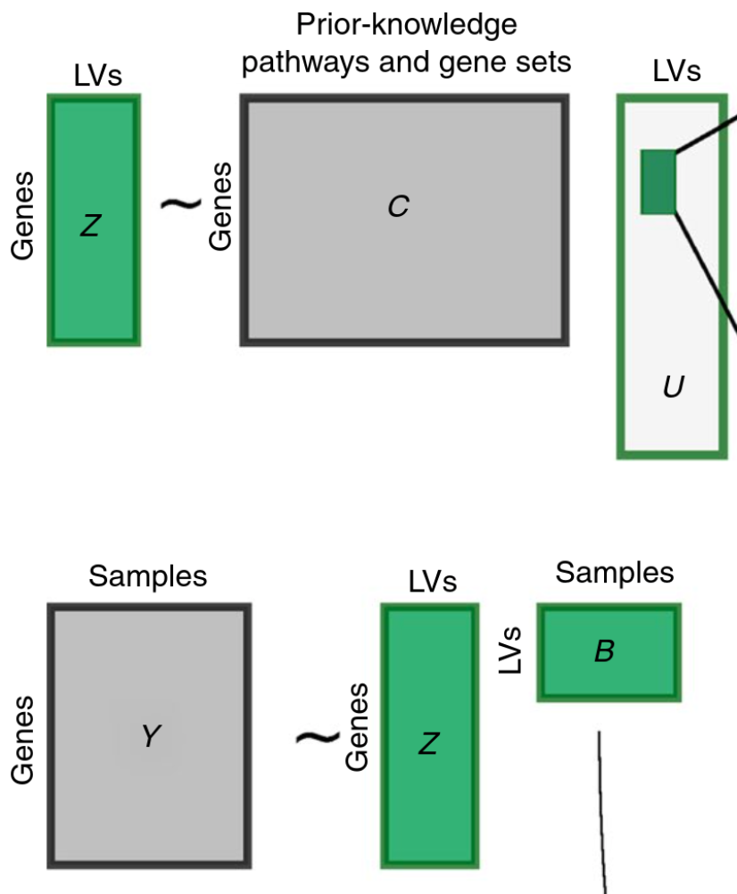
This figure shows what the model learns (green) and uses as input (grey). The rectangles are helpful if you are familiar with linear algebra, but in English, the pieces of the puzzle are:

Inputs:
C - A matrix that describes which genes are in which genesets
Y - The samples of gene expression used to teach the model how gene expression looks

Outputs:
Z - A matrix turns samples of gene expression into latent variables
B - The amount of each latent variable present in each sample
U - Which pathways should be present in each latent variable

PLIER then decides what values each of the outputs should have by optimizing the following equation:

In this section, I’ll go through each term in the equation to explain what is happening.

Reconstruction

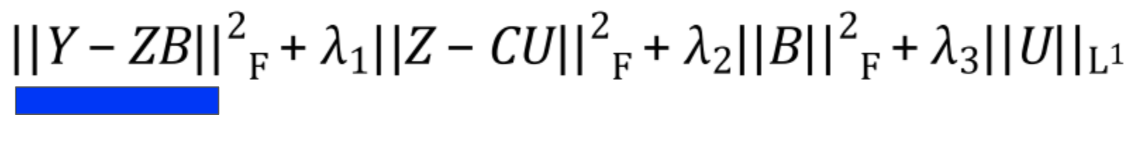
The first term in the equation minimizes reconstruction loss. That is, it minimizes the difference² between the original data and the reconstructed version you get when you convert the data to latent variables and back.

If you’ve read about PCA or SVD, this term will be very familiar. If not, the intuition is that because you’re using a small number of variables to describe the original expression, you often won’t be able to describe it perfectly. The lost information is referred to as the reconstruction error, and we want to minimize it to ensure the variables are good at explaining gene expression.

Pathway Penalty

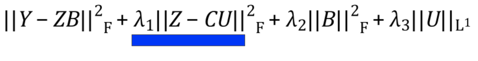
The pathway penalty is PLIER’s secret sauce³. Instead of solely minimizing the reconstruction error like in other matrix factorization methods, PLIER pushes the latent variables to look like the genesets given as prior knowledge.

Latent Variable Regularization

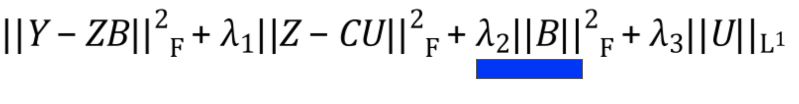
This is a bit of a technical detail, but the latent variables are encouraged to stay small via an L2 norm. There isn’t much of a biological interpretation behind this; it just makes sure that no individual latent variable tries to explain too much of the data.

Geneset Regularization

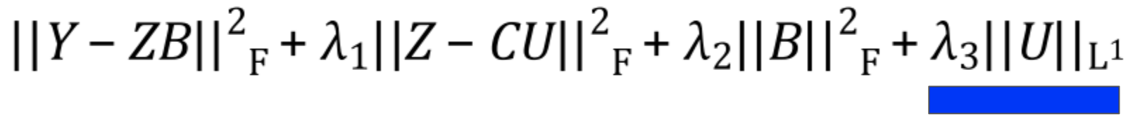
The final term ensures that the pathway matrix is sparse. That is to say that each latent variable should only represent one or a few pathways.

Applying PLIER

Great, now we have a method called PLIER that transforms gene expression into latent variables. How do we use it?

The application of PLIER that I think is most interesting is to learn signals from big datasets and apply them to smaller datasets. One great example of this is the MultiPLIER paper⁴.

The MultiPLIER paper found three main results:

1. You can train a PLIER model on one dataset and learn latent variables that are relevant in another dataset
2. You can train a PLIER model on a compendium of expression data and do as well as or better than a model trained on a tissue-specific dataset
3. You can use the latent variables from a PLIER model trained on a compendium to find signals relevant across tissue types in the same disease

These results open up a lot of potential research directions. For example, MultiPLIER shows that it’s possible to use PLIER for unsupervised transfer learning⁵. As a result, we can avoid some information loss when using PLIER for small data problems by training it on a big dataset first.

Additionally, MultiPLIER shows that PLIER can be helpful to learn more about diseases when using samples from multiple tissues. It can be hard to integrate data from across tissue types due to differences in relevant biological pathways, but PLIER does that for free if it’s trained on a big enough initial dataset.

More concretely, you can run differential expression in latent variable space rather than gene space since you’ll have more power with fewer variables. You can then work backward to determine which biological features the latent variables describe.

Conclusion

You now have a better understanding of PLIER, MultiPLIER, and why they are interesting. Go forth and use this knowledge for good.

Footnotes